Visualizing Real-time Data With STMViewer
If you’ve ever wanted to plot data acquired on your embedded target, this article is for you. It explores common use cases for real-time data visualization using STMViewer. Say goodbye to manual, time-consuming, and error-prone data collection and display methods to speed up your debugging process.
Table of Contents
Why
Visualizing process data in the debugging stage of firmware development offers several advantages - consider a scenario where an embedded controller is responsible for monitoring a physical quantity with a sensor. Plotting the data allows us to validate the accuracy of the recorded measurements and identify any sporadic outliers that may occur. Observing data trends over time can detect other issues, such as excessive noise or deviations in readings, especially those arising under specific conditions. Visualizing can lead to a better understanding of a complex control system’s behavior, as all variables and their interactions can be easily monitored. Additionally, representing specific software actions’ durations and sequences in a digital plot (aka logic analyzer view) can be beneficial when profiling hot code paths or validating the order of asynchronous events.
What exactly can it visualize?
STMViewer consists of two modules which serve a slightly different purpose:
Variable Viewer
Variable Viewer is a module that reads variables’ values directly from RAM using ST-Link SWD (only SWDIO, SWCLK, and GND connection is needed). It is asynchronous, which means it samples the memory with the period set on the PC. It is entirely non-intrusive and can log many variables at once. Writing is supported as well. There are some trade-offs, though. The first one is that logged variables’ addresses must be constant, meaning they must be globals. Moreover, with more aggressive optimization, some variables may get optimized and fail to be logged.
Trace Viewer
Trace Viewer is a module that reads and parses SWO (Serial Wire Viewer) data using an ST-Link. You need to connect SWDIO, SWCLK, SWO, and GND to use it. This tool operates synchronously, meaning it visualizes data points at the rate they are produced on the target. A data point can be either a special single-byte flag used to create digital plots or any value that fits within up to 4 bytes, as in the case of ‘analog’ plots. It incurs minimal performance overhead, involving just a single register write per plot point, as the ITM peripheral handles serialization and timestamping. Trace Viewer can be employed for profiling specific parts of the codebase or visualizing signals that are too fast for the asynchronous Variable Viewer. Its main limitations are the maximum allowed SWO pin baud rate of the ST-Link and that the ITM peripheral is supported only on Cortex M3/M4/M7/M33 cores.
I’m already using STMStudio/CubeMonitor. Why create a new tool?
Let’s begin with the most commonly asked question: Why bother creating a tool when ST provides existing options? There are several reasons:
STMStudio is deprecated, and while it was a helpful tool, it became challenging to work with due to persistent bugs. It also lacks support for mangled C++ names and is exclusively available for Windows.
CubeMonitor, on the other hand, is often considered too much overhead for debugging purposes. It’s primarily designed for creating dashboards, and during debugging, the focus tends to be on functionality rather than aesthetics. Manipulating plot data and writing values to logged variables can be inconvenient. Furthermore, setting up a basic logger configuration can require some time to familiarize with NodeRED’s setup.
Last but not least, none of the available hobby-level software tools include a trace data visualizer. STMViewer’s trace data visualizer is the most intriguing module, enabling users to visualize variables synchronously and profile functions or interrupts within minutes.
Variable Viewer
As mentioned earlier, Variable Viewer is an asynchronous module that samples values from predefined RAM addresses on your target. It can be particularly useful when visualizing multiple, relatively slow signals (with a maximum sampling rate of around 1 kHz). The RAM addresses are read from the project’s *.elf file and parsed using GDB. This is the same approach used by STMStudio and CubeMonitor.
For a quick start, please refer to Variable Viewer.
PID controller
Let’s see Variable Viewer in action on a step response of a classic cascaded PID from a servo drive:
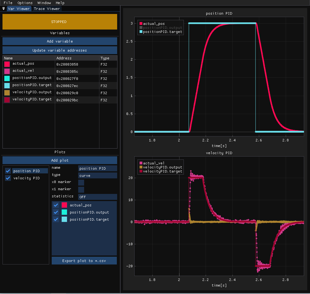
We observe two cascaded controllers: a position PID and a velocity PID. The position PID attempts to follow the target and generates velocity targets for the lower-level controller, which, in turn, generates torque setpoints. When the responses are plotted, it’s easy to notice the overshoots in the velocity PID response, which helps fine-tune the gains. Moreover, we can see when the velocity target limit is being triggered. You can easily measure the most critical parameters of the response using the built-in markers or export a CSV for a more comprehensive analysis.
Trace Viewer
Trace Viewer is a synchronous module used to visualize SWO trace data. This means we can visualize fast actions without worrying some data might be lost between sampling points. It does not require any configuration on the target since it is all done by the STMViewer using SWD. The only thing we have to do is to write data to the ITM->PORT[x] registers to send it. For example:
ITM->PORT[0].u8 = 0xaa; //enter tag 0xaa - plot state high
foo();
ITM->PORT[0].u8 = 0xbb; //exit tag 0xbb - plot state low
can be used to profile a foo() function. Simple, isn’t it? Of course, you can wrap the register writes in a macro, but I wanted to keep it as simple as possible. No extra includes are needed since ITM is defined in CMSIS headers.
On the other hand, this:
float a = sin(10.0f * i);          // some high speed signal to trace
ITM->PORT[0].u32 = *(uint32_t*)&a; // type-punn to desired size: sizeof(float) = sizeof(uint32_t)
can be used to visualize a float value.
Each register write generates two frames on the SWO pin: a data frame and a relative timestamp frame. The data frame holds the channel value, size, and data, while the timestamp frame holds the time elapsed since the last frame, expressed in clock cycles. The variable length of these frames, especially the timestamp frame, makes it very effective in utilizing the available SWO bandwidth. More information on the SWO trace protocol can be found in the Armv7-M Reference Manual1.
For a complete quick start, please refer to Trace Viewer.
Let’s now see a couple of real-life examples.
Profiling function execution time
Let’s check how long it takes to copy a buffer using a well-known memcpy function. I prepared a small demo of ten copy operations, each time 64 bytes larger than the last one:
    volatile uint8_t dest[1024];
    volatile uint8_t src[1024];
    volatile uint16_t size = 1;

    for (size_t i = 0; i < 10; i++)
    {
        ITM->PORT[1].u16 = size;
        ITM->PORT[0].u8 = 0xaa;
        memcpy(dest, src, size);
        ITM->PORT[0].u8 = 0xbb;
        size += 64;

        for (size_t a = 0; a < 300; a++)
            __asm__ volatile("nop");
    }
Besides the memcpy profiling, we also log the current size on channel 1. As can be seen, there is also a small blocking delay to make the plot more readable. Here are the results:
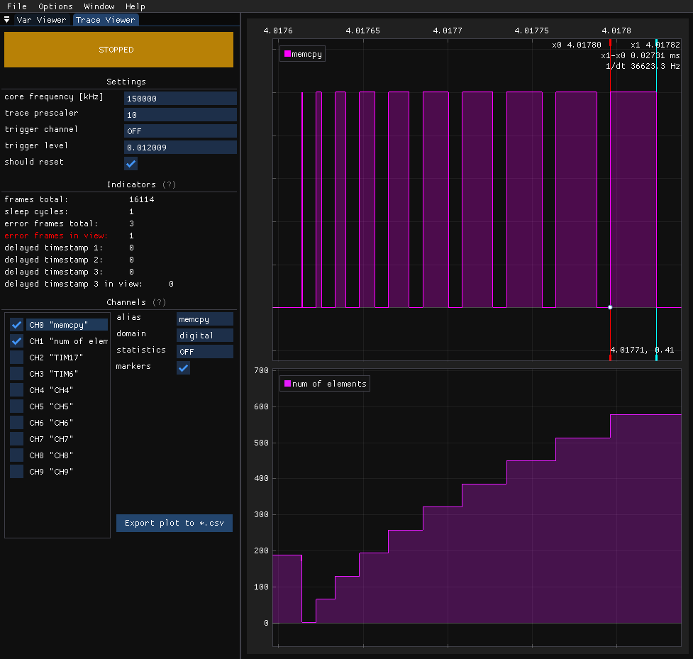
After logging, you can use the markers to determine the time difference between points. Copying a single byte takes about 270 ns, whereas copying 577 bytes takes approximately 25.35 us at 160 MHz.
Profiling multiple interrupts
This example will be similar to the previous one, except we will use multiple channels and try to observe lower-priority interrupts being preempted by higher-priority ones.
I’ve configured three timers and set their interrupt priorities: 0 (highest logical priority) for TIM7, 1 for TIM17, and 2 (lowest) for TIM6. I’ve included some dummy instructions in each interrupt to simulate some work being done.
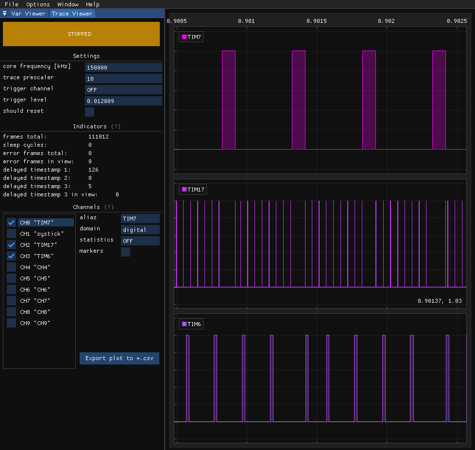
We can observe how the highest priority execution halts all other interrupts, and only after it completes do the other interrupts resume. Particularly significant in such experiments is that the marker register writes used in Trace Viewer are atomic, preventing a higher-priority interrupt between data point generation. This also makes it a valuable tool for visualizing FreeRTOS threads.
High-frequency ADC signal
Have you tried visualizing a high-frequency ADC signal from an embedded target? Some time ago, I had to check the step response of a low-level current controller for a motor. The current was sampled every 25 microseconds, making it quite challenging to visualize. I considered using a DAC and an oscilloscope or recording and replaying the data after the event and eventually went for the latter. Unfortunately, both methods were time-consuming and troublesome.
Let’s see how TraceViewer can handle this task. We will record the current response of an inductor when a voltage step is applied to it:
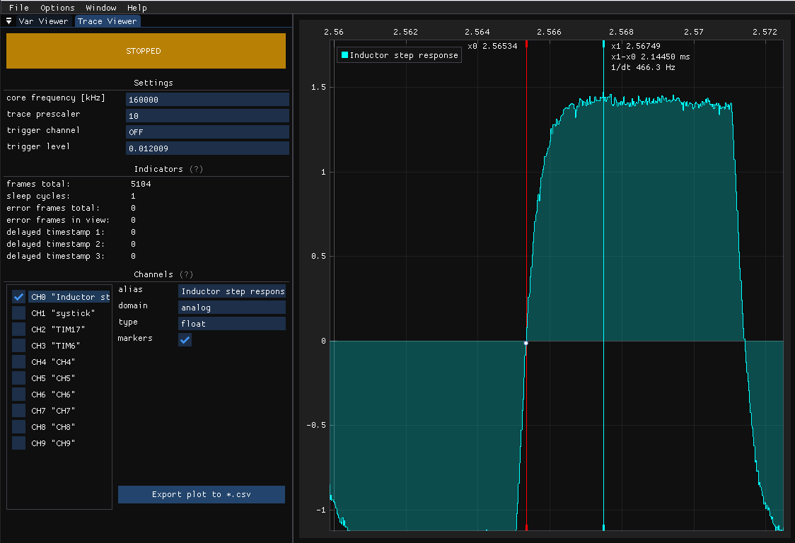
Now, knowing the test voltage, calculating resistance, and measuring rise time, we can easily determine the inductance. No DAC setup or manually collecting the samples was needed!
Conclusion
I hope you find the visual representation of data more appealing after reading this article. Please note that the tool currently only supports the STM32 family. However, if you’d like to join and collaborate on adding support for other microcontrollers and devices, I’d be very happy to do so.
That’s all I have for you today regarding data visualization. I hope you enjoyed it, and if you want to give it a try, check out the releases page on STMViewer’s GitHub.
See anything you'd like to change? Submit a pull request or open an issue on our GitHub
References
 Piotr Wasilewski -- embedded software engineer specializing in motor control applications