Profiling Firmware on Cortex-M
Although microcontrollers in 2020 sometimes come with GHz clock frequencies and even multiple cores, performance is a major concern when developing embedded applications. Indeed, most firmware projects face some real-time constraints which must be carefully managed.
Good profiling tools are therefore essential to firmware development. Historically, profiling was done by toggling GPIOs when specific parts of the code execute. A logic analyzer could then be used to measure the time between different GPIO toggles.
Today, modern microcontrollers implement multiple features to enable advanced profiling techniques. All you need is a debugger and a laptop to get started.
In this post, we explore different techniques that can be used to profile firmware applications running on ARM Cortex-M microcontrollers. To profile our Mandelbrot application on STM32, we start with a naive debugger-based sampling method, and eventually discover ITM, DWT cycle counters, and more!
Table of Contents
Setup
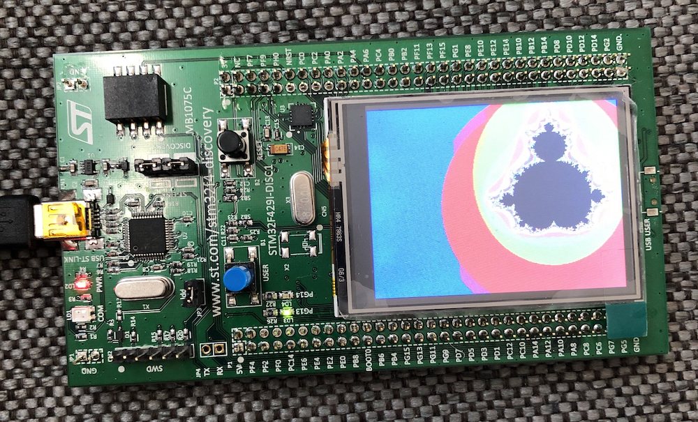
All of the code in this post was written for the STM32F429i Discovery Kit1 by ST Micro. This board is well supported by open source tooling and comes with a built-in STLink debugger with the SWO pin routed through it (more on that later).
As in previous blog posts, we use the excellent openocd tool2 to interface with the board on our laptop. Openocd allows us to flash, debug, and profile the board over USB using the STLink protocol. Since it has built it support for our Discovery board, we simply need to connect our board to our laptop over USB via the “USB-STLINK” port, and run the following command on a recent version of the tool:
$ openocd -f board/stm32f429disc1.cfg
Enabling SWO
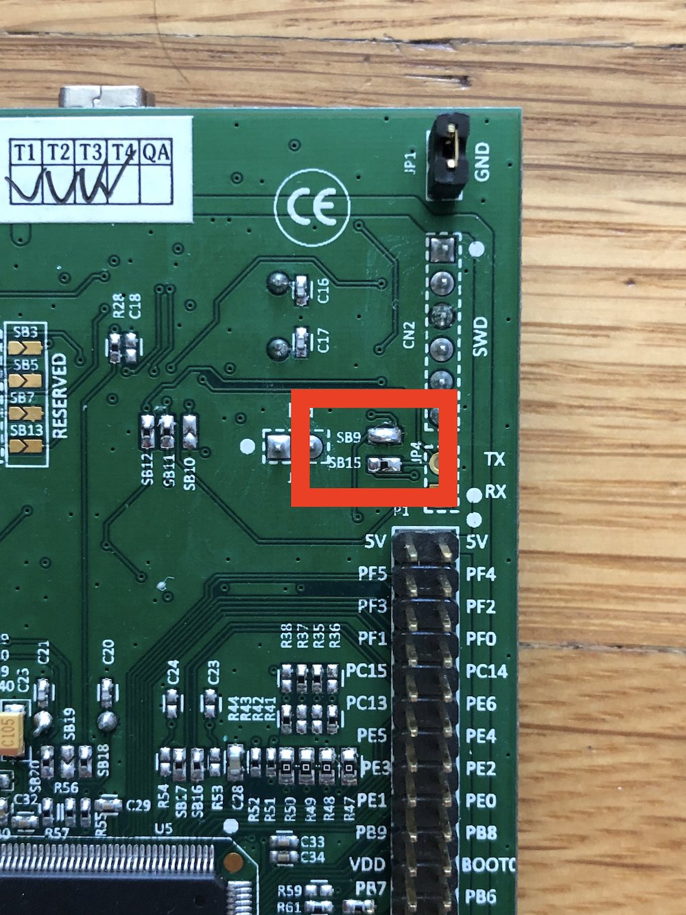
Note that the SWO pin is not connected by default on the Discovery board. Instead, a solder bridge is used to enable the functionality per the User Manual, Section 6.133.
Simply grab a soldering iron and bridge the two pads labeled “SB9” with a bit of solder or a 0-ohm resistor. Here is my handywork:
Code Under Test
In order to have something interesting to profile, we used the Mandelbrot program bundled as an example with libopenCM34. This simple program draws the Mandelbrot fractal on the Discovery board’s LCD screen in a loop. This is CPU intensive and gives us good profiling data.
The example is available on Github.
To clone, build, and flash this example follow these simple steps:
# Clone libopencm3-examples with submodules
$ git clone https://github.com/libopencm3/libopencm3-examples.git --recurse-submodules
...
# Navigate to the Mandelbrot example
$ cd libopencm3-examples/examples/stm32/f4/stm32f429i-discovery/mandelbrot-lcd

# Build the example
$ make
Using ../../../../../libopencm3/ path to library
arm-none-eabi-gcc -Os -std=c99 -ggdb3 -mthumb -mcpu=cortex-m4 -mfloat-abi=hard -mfpu=fpv4-sp-d16 -Wextra -Wshadow -Wimplicit-function-declaration -Wredundant-decls -Wmissing-prototypes -Wstrict-prototypes -fno-common -ffunction-sections -fdata-sections  -MD -Wall -Wundef -DSTM32F4 -I../../../../../libopencm3//include  -o sdram.o -c sdram.c
arm-none-eabi-gcc -Os -std=c99 -ggdb3 -mthumb -mcpu=cortex-m4 -mfloat-abi=hard -mfpu=fpv4-sp-d16 -Wextra -Wshadow -Wimplicit-function-declaration -Wredundant-decls -Wmissing-prototypes -Wstrict-prototypes -fno-common -ffunction-sections -fdata-sections  -MD -Wall -Wundef -DSTM32F4 -I../../../../../libopencm3//include  -o lcd.o -c lcd.c
arm-none-eabi-gcc -Os -std=c99 -ggdb3 -mthumb -mcpu=cortex-m4 -mfloat-abi=hard -mfpu=fpv4-sp-d16 -Wextra -Wshadow -Wimplicit-function-declaration -Wredundant-decls -Wmissing-prototypes -Wstrict-prototypes -fno-common -ffunction-sections -fdata-sections  -MD -Wall -Wundef -DSTM32F4 -I../../../../../libopencm3//include  -o clock.o -c clock.c
arm-none-eabi-gcc -Os -std=c99 -ggdb3 -mthumb -mcpu=cortex-m4 -mfloat-abi=hard -mfpu=fpv4-sp-d16 -Wextra -Wshadow -Wimplicit-function-declaration -Wredundant-decls -Wmissing-prototypes -Wstrict-prototypes -fno-common -ffunction-sections -fdata-sections  -MD -Wall -Wundef -DSTM32F4 -I../../../../../libopencm3//include  -o mandel.o -c mandel.c
arm-none-eabi-gcc --static -nostartfiles -T../stm32f429i-discovery.ld -mthumb -mcpu=cortex-m4 -mfloat-abi=hard -mfpu=fpv4-sp-d16 -ggdb3 -Wl,-Map=mandel.map -Wl,--cref -Wl,--gc-sections -L../../../../../libopencm3//lib sdram.o lcd.o clock.o mandel.o -lopencm3_stm32f4 -Wl,--start-group -lc -lgcc -lnosys -Wl,--end-group -o mandel.elf

# start GDB
$ arm-none-eabi-gdb mandel.elf

# Connect to OpenOCD (it must already be running in another terminal)
(gdb) target remote :3333

# Reset & Halt the target
(gdb) monitor reset halt

# Flash the firmware
(gdb) load

# Start the firmware
(gdb) continue
You should now be seeing the Mandelbrot fractal on the LCD of the Discovery board. Here it is!
Poor Man’s Profiler
The simplest way to profile a system is to use a sampling profiler. The concept is simple: record the program counter at regular intervals for a period of time. Given a high enough sampling rate for a long enough duration, you get a statistical distribution of what code is running on your device.
One of the main advantages of sampling profilers is that they do not require modifying the code you are trying to inspect. Other approaches like instrumenting your code can yield more precise results, but risk changing the behavior of the program.
So how can we sample our program counter at a regular interval? Using our debugger! This is a common approach, sometimes dubbed the poor man’s profiler.
The concept is simple: we write a script which executes our debugger in a loop and dumps the current backtrace. After we’ve collected enough data points, we parse the backtraces and match them up to get aggregate values.
To do this we must run arm-none-eabi-gdb in batch mode: we want it to start,
connect, run our command, and exit without user input. This is supported with the
-batch flag. Here’s the invocation:
$ arm-none-eabi-gdb -ex "set pagination off" -ex "target remote :3333" -ex "thread apply all bt" -batch $elf
This will start GDB, disable pagination (it requires user input), run target
remote :3333 to connect to OpenOCD, run thread apply all bt to get the
backtrace of every thread, and exits.
To parse the data, I’ve adapted the awk script provided at
poormansprofiler.org to handle the specific output of arm-none-eabi-gdb.
Altogether this gives us the following:
#!/bin/bash
nsamples=1000
sleeptime=0
elf=mandel.elf

for x in $(seq 1 $nsamples)
  do
    arm-none-eabi-gdb -ex "set pagination off" -ex "target remote :3333" -ex "thread apply all bt" -batch $elf
    sleep $sleeptime
  done | \
awk '
  BEGIN { s = ""; }
  /^Thread/ { print s; s = ""; }
  /^\#/ {
      if (s != "" ) { if ($3 == "in") {  s = s "," $4 } else {  s = s "," $2 }}
      else { if ($3 == "in") {  s = $4 } else {  s = $2 } }
  }
  END { print s }' | \
sort | uniq -c | sort -r -n -k 1,1
Running this script, we get the following output:
$ sh pmp.sh
 592 spi_xfer,lcd_command,??
 408 spi_xfer,lcd_command,lcd_show_frame,main
   1
Using these initial results, it appears that we spend most of our time sending frames to the LCD over SPI.
Unfortunately, we cannot get much more precise results using this approach. Using GDB and OpenOCD introduces huge overhead, which means that we are limited to a datapoint every 50ms. Given that our MPU executes on the order of 200 million clock cycles per second, that means that we get a sample every 10 million clock cycles. This is too coarse for any meaningful analysis, so we must find a better approach
PC Sampling with ITM
To get better profiling data, we turn to the Instrumented Trace Macrocell (ITM). The ITM is an optional feature of ARM Cortex-M cores which formats and outputs trace information generated by the firmware or directly from the hardware over a dedicated bus.
Note: ITM is not available on Cortex-M0, M0+, and M23 based microcontrollers.
Typically ITM is used to print out debug data from firmware, much like one would
use printf over a serial bus. ITM is strictly superior to UART in this case as
it is faster, works directly with your SWD adapter, and is buffered so the CPU
does not need to wait. You can read more about using ITM for logging in Jorge
Aparicio’s excellent post on the topic.
Where ITM really shines is its ability to output data generated directly by the hardware. As of this writing, ITM supports the following hardware data sources:
- Event counter wrapping: When enabled, an event is generated when DWT event counters overflow. This includes clock cycle counters, folded instruction counters, sleep cycle counters, and more5.
- Exception tracing: When enabled, an event is generated whenever an exception (i.e. Interrupt) occurs.
- PC sampling: When enabled, an event is generated at a regular interval containing the current PC.
- DWT Data trace: When enabled, events are generated when a specific data address (or range of addresses) is accessed. The events contain the PC, the data address, and the data value.
This information can be read over the TRACE pins of your MCU if you have a trace-enabled debugger (e.g. a J-Trace or a Lauterbach TRACE32), alternatively it can be streamed over the SWO pin of your SWD bus. While more pins allow for more data to be read, much can be done with the single SWO pin without requiring complex tools.
Note: Using ITM for printf is relatively straightforward. Here’s a putc implementation that should do the trick:
void putc(char c) {
  while (ITM_STIM32(0) == 0);
  ITM_STIM8(0) = c;
}
You can then just
cattheitm.fifofile we configure with openOCD below and see the print output. It’s pretty cool!
Enabling PC Sampling with ITM and OpenOCD
You will notice that “PC Sampling” is explicitly called out as one of the things we can do with ITM. With ITM PC Sampling, we can build a much better Sampling Profiler!
Configuring OpenOCD
First, we must configure OpenOCD to read from the SWO pin and dump the data
somewhere we can read it. This is done via the tpiu config
command6. This command configures the Trace Port Interface
Unit[^tpiu] in the chip and enables saving to file in openOCD. I’ve summarized
it below:
tpiu config (disable | ((external | internal (filename | -)) (sync port_width | ((manchester | uart) formatter_enable)) TRACECLKIN_freq [trace_freq]))
Here is what we want to do here:
- Set TRACELCKIN_FREQ to our core frequency (168MHz for the STM32F429). This is important as you will get corrupted data on your SWO pin otherwise.
- Redirect the ITM data to a file with
internal <filename>. Usingexternalwould require we use an adapter to read the data directly from the pin with e.g. a UART to USB adapter - Use UART rather than Manchester encoding to make it easy to decode the data
From GDB, we use monitor to send commands to OpenOCD, so we get the following command:
(gdb) monitor tpiu config internal itm.fifo uart off 168000000
Enabling PC Sampling Events
Next, we configure our MCU to output PC Sampling events. This is done using the
DWT Control Register. The register is at address 0xE0001000, I’ve reproduced
its layout below:
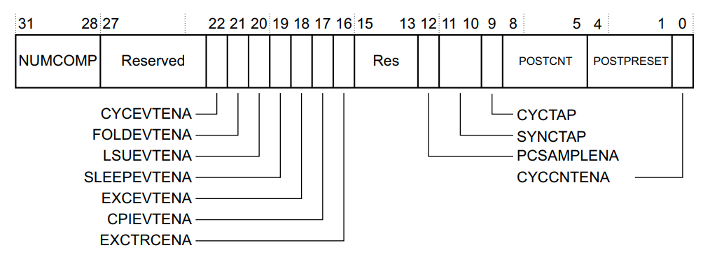
For our use case, we care about the following bits:
- Bit 12: PCSAMPLEENA. Setting this to 1 will enable PC sampling events.
- Bit 0: CYCCNTENA. This enables the CYCCNT counter which is required for PC sampling.
- Bit 9: CYCTAP. This selects which bit in the cycle counter is used to trigger PC sampling events. A 1 selects bit 10 to tap, a 0 selects bit 6 to tap.
- Bits 1-4: POSTPRESET. These bits control how many times the time bit must toggle before a PC sample event is generated.
Let me explain how the system works: CYCCNTENA enables a cycle counter in the DWT unit of your microcontroller. This counter is incremented every CPU cycle (i.e. 168 million times per second). Whenever the CYCTAP bit in the cycle counter is toggled (0->1 or 1->0), we decrement a counter which started at the POSTPRESET value. When that counter hits 0, a PC sampling event is generated.
Here’s a practical example: if CYCTAP is set to 0 and POSTPRESET is set to 4, we tap the 6th bit of the cycle counter. This means that the tap is toggled every 64 (or 2^6) cycles. After 4 tap toggles, a PC sample event is generated which works out to 256 (4 * 64) cycles. In other words, the PC sampling rate is 0.65MHz (168MHz / 256).
We are limited by the speed of our debug adapter, so in my case, I tapped the 10th bit (CYCTAP = 1), and set POPRESET to 3. This means that we are sampling the PC every 3,072 cycles, or at 50KHz.
Using OpenOCD, we write the register so that PCSAMPLEENA = 1, CYCCNTENA = 1, CYCTAP = 1, and POSTPRESET = 3. This requires the following command:
(gdb) monitor mww 0xE0001000 0x1207 0x103FF
Last but not least, we enable ITM port 0 which is a built in openOCD feature:
(gdb) monitor itm port 0 on
Decoding ITM Data
If all went well, we now have a file named itm.fifo which contains binary ITM
data. We must now decode it!
The packet format is specified in detail in the ARM v7m Architecture Reference Manual. Thankfully, others have gone through the trouble of implementing decoders for us.
My favorite tool here is the itm-tools suite from Jorge Aparicio, which is
available on Github. You will need a
relatively recent Rust toolchain to compile it.
In case you are not familiar with Rust, here are simple steps to run to get the tools:
$ git clone https://github.com/japaric/itm-tools
...
$ cd itm-tools
$ cargo build
...
   Compiling addr2line v0.12.1
   Compiling backtrace v0.3.48
   Compiling synstructure v0.12.3
   Compiling failure v0.1.8
   Compiling exitfailure v0.5.1
   Compiling itm v0.4.0 (https://github.com/rust-embedded/itm#9298d128)
   Compiling itm-tools v0.1.0 (/Users/francois/code/itm-tools)
    Finished dev [unoptimized + debuginfo] target(s) in 50.20s
You will then find the itm-decode and pcsampl programs under target/debug.
First, we can use itm-decode to verify our ITM data contains the PC samples we
expect:
$ ~/code/itm-tools/target/debug/itm-decode itm.fifo 2>/dev/null
...
PeriodicPcSample { pc: Some(134219118) }
PeriodicPcSample { pc: Some(134219084) }
PeriodicPcSample { pc: Some(134219106) }
PeriodicPcSample { pc: Some(134219072) }
PeriodicPcSample { pc: Some(134219084) }
PeriodicPcSample { pc: Some(134219106) }
PeriodicPcSample { pc: Some(134219072) }
PeriodicPcSample { pc: Some(134219084) }
PeriodicPcSample { pc: Some(134219106) }
PeriodicPcSample { pc: Some(134219118) }
PeriodicPcSample { pc: Some(134219084) }
PeriodicPcSample { pc: Some(134219094) }
PeriodicPcSample { pc: Some(134219106) }
PeriodicPcSample { pc: Some(134219072) }
PeriodicPcSample { pc: Some(134219084) }
PeriodicPcSample { pc: Some(134219094) }
PeriodicPcSample { pc: Some(134219106) }
That looks great! Note that if you see too many Overflow packets your debug
adapter is not able to keep up with your sampling rate and you should increase
the POSTPRESET value in the DWT Control Register to lower the sampling rate.
Next, we can use the pcsampl utility to analyze the profiling data:
$ ~/code/itm-tools/target/debug/pcsampl itm.fifo -e mandel.elf 2>/dev/null
    % FUNCTION
 0.05 *SLEEP*
51.94 mandel
32.64 spi_xfer
 8.40 lcd_command
 4.63 lcd_draw_pixel
 2.17 msleep
 0.10 uart_putc
 0.02 _realloc_r
 0.01 rcc_clock_setup_pll
 0.01 sys_tick_handler
 0.00 __fputwc
 0.00 _fclose_r
 0.00 __sfvwrite_r
 0.00 gpio_mode_setup
 0.00 _dtoa_r
-----
 100% 23170 samples
As you can see, this data is much more detailed than what we got with the Poor
Man’s Profiler approach. In fact, we can see that we are spending most of our
time in the mandel function, and not in the spi_xfer function as we
thought.
Note: In the process of writing this blog post, I stumbled upon the Orbuculum project. While this looks very promising for ITM/ETM and other debugging, I was not able to get it to work on MacOS.
Profiling Individual Functions
So far, we have been profiling our entire program. This is useful to identify overall bottlenecks, but oftentimes we are concerned only with a specific code path. For example, we may want to profile a specific message parser, or an interrupt service routine.
To do this, we will need to modify our firmware code a bit. Our goal is to write
a PROFILE macro which can be used to enable ITM profiling for a specific set
of code.
In our Mandelbrot example, let’s profile lcd_show_frame. We want our macro to
be invoked as such:
int main(void) {
    ...
    PROFILE(lcd_show_frame());
    ...
}
What does our macro need to do? At a high level:
- Enable PC sampling
- Execute the code being profiled
- Disable PC sampling
We can start filling in our macro:
#define PROFILE(code) {         \
  // enable PC sampling         \
  code;                          \
  // disable PC sampling        \
}
To enable or disable PC sampling, we need to write to the DWT Control Register. Thankfully, libopencm3 has a definition for this register7 and its fields which makes our life easy.
To enable PC sampling:
DWT_CTRL &= ~DWT_CTRL_POSTPRESET;
DWT_CTRL |= 0x3 << DWT_CTRL_POSTPRESET_SHIFT;
DWT_CTRL |= DWT_CTRL_CYCTAP;
DWT_CTRL |= DWT_CTRL_PCSAMPLENA;
and to disable it:
DWT_CTRL &= ~DWT_CTRL_POSTPRESET;
DWT_CTRL &= ~DWT_CTRL_CYCTAP;
DWT_CTRL &= ~DWT_CTRL_PCSAMPLENA;
We wrap this into a function to make our life easier:
static void dwt_pcsampler_enable(bool enable) {
    if (enable) {
        DWT_CTRL &= ~DWT_CTRL_POSTPRESET;
        DWT_CTRL |= 0x3 << DWT_CTRL_POSTPRESET_SHIFT;
        DWT_CTRL |= DWT_CTRL_CYCTAP;
        DWT_CTRL |= DWT_CTRL_PCSAMPLENA;
    } else {
        DWT_CTRL &= ~DWT_CTRL_POSTPRESET;
        DWT_CTRL &= ~DWT_CTRL_CYCTAP;
        DWT_CTRL &= ~DWT_CTRL_PCSAMPLENA;
    }
}
and fill in our macro:
#define PROFILE(code)                   \
    {                                   \
        dwt_pcsampler_enable(true);     \
        code;                            \
        dwt_pcsampler_enable(false);    \
    }
That was easy! We now have a PROFILE macro we can use to profile an individual
function. Note that this macro can only be used to profile a single function at
a time since there does not appear to be a way to set an ITM port for PC
sampling data.
Let’s rebuild our firmware, collect some data:
$ make
$ arm-none-eabi-gdb mandel.elf
...
For help, type "help".
Type "apropos word" to search for commands related to "word"...
Reading symbols from mandel.elf...

(gdb) target remote :3333
Remote debugging using :3333
iterate (py=1.00990558, px=<optimized out>) at mandel.c:121
121                     it++;
(gdb) mon reset halt
target halted due to debug-request, current mode: Thread
xPSR: 0x01000000 pc: 0x08000c68 msp: 0x20030000
(gdb) load
Loading section .text, size 0x6ea0 lma 0x8000000
Loading section .ARM.exidx, size 0x8 lma 0x8006ea0
Loading section .data, size 0xa1c lma 0x8006ea8
Start address 0x8000ca4, load size 30916
Transfer rate: 26 KB/sec, 7729 bytes/write.
(gdb) monitor tpiu config internal itm.fifo uart off 168000000
(gdb) monitor itm port 0 on
(gdb) continue
Continuing.
This will generate some more ITM data, but this time only for our function under
test. After running this for a little bit we can run pcsampl on the new data
file:
$ ~/code/itm-tools/target/debug/pcsampl itm.fifo -e mandel.elf 2>/dev/null
    % FUNCTION
 0.00 *SLEEP*
79.27 spi_xfer
19.20 lcd_command
 1.25 msleep
 0.17 mandel
 0.08 lcd_draw_pixel
 0.01 sys_tick_handler
 0.01 rcc_clock_setup_pll
 0.01 lcd_show_frame
 0.00 gpio_set_output_options
 0.00 _vfprintf_r
-----
 100% 39863 samples
As you can see, we now see the breakdown of time spent within lcd_show_frame,
and as expected spi_xfer takes the lion’s share.
Note: this approach is not perfect. Since IRQs are running, the function we are trying to profile could get interrupted which means we will collect some samples from other parts of our code as well. In a single threaded program, this is not a huge deal but can be more problematic when multiple threads are running and pre-empting each other.
Timing Code With the Cycle Counter
Our sampling profiler is able to tell us the relative time spent in one
function versus another. However, it does not tell us anything about absolute
time spent. If we want to optimize our mandel function, we will need a way to
measure how long it executes for.
This is where the CYCCNT register (address: 0xE0001004) comes in. As noted
earlier, the cycle counter is a free running 32-bit cycle counter which is used
to tee-off PC sampling events. The cycle counter can also be used to measure
time without needing to use a hardware timer.
To use the CYCCNT to time a function, we simply need to read it before and
after the function executes, and compute the delta.
Note: since the CYCCNT register is 32-bit wide, it can not be used to measure time periods longer than
cycle_period* 2^32. Given our 168MHz clock speed, this comes to about ~25 seconds in our case.
We already know how to enable the cycle counter: we set the CYCCNTENA bit in the DWT Control Register (this was required for PC sampling as well).
void enable_cycle_counter(void) {
    DWT_CTRL |= DWT_CTRL_CYCCNTENA;
}
To read the cycle counter we simple read that register:
uint32_t read_cycle_counter(void) {
    return DWT_CYCCNT;
}
That’s it! Now we can measure the time spent in our mandel function as such:
int main(void) {
    ...
    enable_cycle_counter(); // << Enable Cycle Counter
    printf("System initialized.\n");
    while (1) {
        uint32_t start = read_cycle_counter(); // << Start count
        mandel(center_x, center_y, scale);	/* draw mandelbrot */
        uint32_t stop = read_cycle_counter(); // << Stop count
        printf("We spent %lu cycles in mandel\n", stop - start);
        ...
    }

    return 0;
}
Note: libopencm3 has APIs to use the cycle counter already implemented:
dwt_enable_cycle_counteranddwt_read_cycle_counter. I chose to implement them myself to make it easier to reproduce for those who do not use the library.
And here are the results:
...
We spent 23392491 cycles in mandel
We spent 24345217 cycles in mandel
We spent 25360211 cycles in mandel
We spent 26309694 cycles in mandel
We spent 27019451 cycles in mandel
We spent 27434047 cycles in mandel
We spent 27662784 cycles in mandel
We spent 27868860 cycles in mandel
We spent 28259158 cycles in mandel
We spent 28544329 cycles in mandel
We spent 28927996 cycles in mandel
We spent 29792795 cycles in mandel
We spent 30591276 cycles in mandel
We spent 31332753 cycles in mandel
We spent 32102420 cycles in mandel
We spent 32874457 cycles in mandel
We spent 33490363 cycles in mandel
We spent 33849665 cycles in mandel
We spent 34146071 cycles in mandel
We spent 34523587 cycles in mandel
We spent 34923967 cycles in mandel
We spent 35274893 cycles in mandel
We spent 35667430 cycles in mandel
We spent 36211229 cycles in mandel
We spent 36762744 cycles in mandel
We spent 37389846 cycles in mandel
We spent 37976133 cycles in mandel
We spent 38298322 cycles in mandel
We see here that the amount of time spent in the mandel function increases
with every iteration. To convert cycles to seconds we simply divide by our clock
frequency. e.g. 38298322 cycles works out to ~23ms at 168MHz.
Note: You can find libraries on Github that implement a bit more logic on top of the cycle counter, so multiple functions can be measured within the same run. Here are two that I stumbled upon while researching this article: https://github.com/Serj-Bashlayev/STM32_Profiler, and https://github.com/esynr3z/profiler-cortex-m4.
Closing
I hope this post gave you a better understanding of the profiling features available on Cortex-M microcontrollers. I am amazed at what can be accomplished with an open source tool such as openOCD and a single pin!
Are there profiling tools or methods you’ve used to great effect? Let us know in the comments below!
See anything you'd like to change? Submit a pull request or open an issue on our GitHub
References
-
More information on getting OpenOCD at http://openocd.org. ↩
-
You can read more about DWT counters on ARM’s Website ↩
 François Baldassari has worked on the embedded software teams at Sun, Pebble, and Oculus. He is currently the CEO of Memfault.